请问有谁知道关于光学传递函数的书?
麻烦推荐一下.
TKS!| 出版年 | |||||
| 1 | 光学传递函数 | 庄松林 | 机械工业出版社 | 1981 | |
| 2 | 光学传递函数及其数理基础 | 麦伟麟 | 国防工业出版社 | 1979 | |
| 3 | 光学传递函数术语,符号GB4315-84 | 中国标准出版社 | 1984 | ||
| 4 | 光学传递函数数学基础 | 孙树本 | 科学出版社 | 1980 |
感謝那

感谢啊
应该是一些矩阵
国内的书太专业了,都是高数公式的堆积,有兴趣的看一下英文的解释,比较浅显易懂,关键是和实际结合的好!可惜有些图片不知怎样传上去
Introduction
Modulation Transfer Function (MTF) is the scientific means of evaluating the fundamental spatial resolution performance of an imaging system, or components of that system. The purpose of this article is to introduce the MTF concept and its use, and to show why it is a superior way of specifying spatial resolution compared to other methods such as dots-per-inch (dpi) or visual bar target readings.
What is Resolution and How Does it Relate to MTF?
Resolution is a measure of how well spatial details are preserved. The measuring of two items are required to define it: (1) spatial detail and (2) preservation. It is these fundamental metrics of detail and preservation that define MTF.
Detail and preservation metrics are not single measurements, but rather a continuum of measurements, which is why a functional curve quantifying them, i.e., the MTF, can be plotted. A range of spatial details is characterized by how well each and every one of those details is preserved, some better than others. An entire set of point pairs are then plotted - a measure of spatial detail or "frequency" on the x-axis and "extent of preservation" of that detail on the y-axis - to form the MTF as illustrated in Figure 1.
One of the beauties of MTF is that it provides a continuum of unique rankings by which to judge a device's resolution performance. For the indecisive this may pose a problem, but for the analyst, this is gold.
How is MTF Measured?
As stated above, two items are required for defining the MTF: (1) a measure of spatial detail, called frequency, and (2) a fundamental measure for determining how that detail is preserved, called modulation transfer. These will be addressed in that order.
Frequency - Spatial detail can be measured by the spatial frequency content of a given feature. A good example of this is the frequency of the line features in any 5 line bar target group. Each of the labeled line groups in a target indicates the spatial frequency for that group. For instance, the group labeled 2.0 has a frequency of 2.0 line pairs per millimeter (2.0 lp/mm). A line pair (dark-line/white-space combination) is more universally referred to as one cycle. For this example then, one cycle (line pair) spans 1/2.0 = 0.50 mm. The higher the frequency, the greater the detail, the greater the number of cycles per unit distance, and the more closely spaced the lines become.
In scientific lexicon, the lines in the bar target cited above are called square-wave signals. This term derives from the square corners of their light intensity profile, as shown in the left hand side of Figure 2 below. Though square wave signals are easy to manufacture into targets and can be used to measure MTF when properly treated, alone, they are not considered to be basic image building blocks. As such it is technically incorrect to use them as reference signals in determining MTFs. Instead, sine-waves are used. An example of a sine-wave signal compared with a square-wave of the same frequency is also shown in Figure 2. Below each image is a cross-section plot of their light intensity profiles.
cross-section direction -------------------------------------------------------------------------------
Sine-wave frequencies, usually in units of cycles/mm, are used as the metric for specifying detail in an MTF plot. These frequencies are always plotted as the independent variable on the x-axis. To complete the MTF metric, a measure of how well each sine-wave frequency is preserved after being imaged, i.e., transferred through an imaging device, is required. This measure, called modulation transfer, is plotted along the y-axis for each available frequency and completes the specification of MTF.
Modulation Transfer - The modulation for any signal is defined with two variables of that signal, the maximum light intensity value, Imax, and minimum light intensity value, Imin. Modulation is formulated as the quotient of their differences to their sums, as follows:
Modulation = (Imax - Imin)/ (Imax + Imin)
Figure 3 illustrates its calculation for a sine-wave signal of 70% modulation. Note that its calculation is done in light reflectance, not density. Reflectance is considered a proper linear space in which to make the calculation.
The goal in determining MTF is to measure how well the input modulation is preserved after being imaged or in some way acted upon. This modulation transfer is quantified by comparing the modulations of the output sine-waves after being imaged to the target's input sine-wave modulations before being imaged. This comparison is a simple ratio of output modulation to input modulation. It is formulated as:
Modulation Transfer = (Output Modulation)/ (Input Modulation) = (Mo) /(Mi
The modulation transfer calculation is now complete. For a number of known frequencies, f, with known input modulations, Mi, an output modulation, Mo, can be determined after imaging. The ratio of Mo/Mi is then plotted for each frequency. The resulting curve is the Modulation Transfer Function, or MTF. It is also sometimes called the Signal Frequency Response, or SFR.
An Example
Suppose one wished to determine the MTF of a desktop document scanner. A straightforward way of doing this is through the use of a sine-wave target. A good one will have a range of sine-wave frequencies along with solid gray patch areas used for calibration. The target will come with supporting literature regarding the frequencies of each sine-wave, their modulation, and the reflectances of the gray patches
One would place the target on the platen, ensure it is properly aligned, choose a scanning resolution, and perform an 8-bit/channel (256 gray levels) scan. One now has a digital image of that target with potential count values ranging from 0 through 255 for each color channel. The calibration patches would then be used to ensure that the data was linear with respect to count value. For simplicity, the green channel alone will be analyzed. With a digital image analysis program, such as Adobe Photoshop®, one would determine the average minimum and average maximum count value associated with the darkest and lightest areas of each sine-wave frequency. These minimum and maximum count values are used to determine the output modulation, Mo, for each of the available frequencies. The modulation transfer would then be calculated. In tabular form these calculations appear as follows.
Frequency (cycles/mm) | Target Modulation (Mi) | Avg Max. count value (out | Avg. Min.count value (out | Output Modulation (Mo)
| Modulation Transfer (Mo/Mi) |
1.0 | 0.70 | 254 | 46 | 0.69 | 0.98 |
3.0 | 0.70 | 234 | 66 | 0.56 | 0.85 |
5.0 | 0.65 | 201 | 99 | 0.34 | 0.53 |
6.0 | 0.63 | 187 | 112 | 0.25 | 0.40 |
7.0 | 0.58 | 170 | 130 | 0.13 | 0.22 |
9.0 | 0.55 | 154 | 145 | 0.03 | 0.06 |
10.0 | 0.50 | 153 | 147 | 0.02 | 0.03 |
11.0 | 0.46 | 151 | 148 | 0.01 | 0.02 |
12.0
| 0.44 | 150 | 150 | 0.00 | 0.00 |
|
|
|
|
|
|
A plot of Modulation Transfer vs. Frequency yields the MTF for the scanner with the selected settings (i.e., dpi, sharpening, bit depth, etc.) as illustrated in Figure 4 below.
How is the MTF Curve Interpreted?
The MTF shape of Figure 4 is typical for a well-behaved optical imaging device such as a document scanner. It begins with near unity modulation at zero-frequency and gradually becomes lower towards higher frequencies, until at some point the modulation becomes zero and remains so for all higher frequencies.
A simple way to interpret the modulation transfer is by thinking of it as a measure of how well the scanner preserves the average contrast of each input sine-wave frequency. A modulation transfer of 1 indicates that the average contrast for a given sine-wave frequency is perfectly maintained, while zero modulation transfer shows that it was completely lost, or not "seen" in the imaging process. Values between 0-1 indicate varying degrees of contrast preservation. Though there are exceptions, generally, the higher the modulation transfer, the better the preservation of detail by the imaging system.
Perhaps the best way to become grounded in interpreting MTF is through the use of example images captured using scanners with various MTFs. Figure 5 shows such an example for a section of an RIT Alphanumeric Resolution Test Object. (1)
The MTFs for each of the optical systems through which the target was imaged are labeled in the MTF plots below the image. Though the majority of the character sets are readable, their degree of legibility is quite different. The spatial image quality of the image on the right is superior to its two neighbors, and the middle one is superior to its left neighbor. This difference is reflected in the shape of the MTF. Figure 5 also illustrates why limiting resolution metrics derived from visual evaluations of classical targets of bars, characters, or other square wave-like features often fall short as spatial resolution tools.
Why is MTF Better Than Other Resolution Measures?
Limiting Resolution - If one were to use a limiting resolution technique, such as visual bar target readings on the examples of Figure 5, each image would be rated the same since the smallest or limiting character group that can be just visually detected in each would be the "25E" group (near the bottom of the white square). These visual judgments of limiting resolution are considered threshold metrics because they rely on judgments of the threshold at which spatial resolution breaks down, and not the way it performs in getting to that threshhold. Though useful in statistical analyses, one-bit imagery, and noise-limited imaging, limiting resolution is not considered fundamental for resolution measurement. The three imaging systems illustrated in Figure 5 would have been judged equivalent with a limiting resolution metric. It is clear that they are not the same in terms of character image quality.
Dots Per Inch - For completeness, a few words on why specifying resolution of digital scanners in terms of dpi is misleading. The addressable resolution, specified in dots-per-inch (dpi), is marginally useful for evaluating true scanner resolution, but is only an indication of the sampling interval between pixels. It is not an indication of what size detail the scanner can ultimately see, or its MTF behavior, as much as it is of how finely the center of a pixel can be located.
For instance, it is reasonable to assume that a 400 dpi scanner will precisely sample a scanned document every 1/400". It is not reasonable to assume, however, that it will actually "see" details this small. It may be able to detect details only as fine as a good 300 dpi scanner. In fact, for most desktop document scanners, the disparity between the sampling interval and actual detail detection becomes highly probable for claimed addressable resolutions beyond 1000 dpi.
Relying on dpi is like trying to compare the passing of either a needle (small cross section) or a large nail (large cross section) through common door screening. Although both can be accurately located at any screen opening, because of its small size, only the needle will make it through. The same can be said of a digital document scanner. The sampling interval (screen spacing) does not determine how large or small an area that the scanner can see, but only how frequently it sees it.
Imaging System Analysis - Perhaps the single biggest benefit of using MTFs is for their utility in evaluating systems of connected imaging components. Besides the example of a scanner used in this paper, other system components, such as image processing, human vision, and information display, can also be cast in terms of MTF performance. Because MTF measurements are fundamental, the MTFs of these individual components can be cascaded to predict the way that a system of components will perform as a unit in terms of spatial resolution.
Conclusion
At a recent digitizing conference, one of the more prestigious speakers proclaimed, "Resolution is dead!" The message was that resolution was well understood with the real future challenge being consistent color reproduction. While the latter is no doubt a big hurdle, the trivializing of measuring spatial resolution as if it were a fashion trend is unfortunate, especially considering that most practitioners' understanding of resolution stops at either limiting resolution or addressable resolution. The truly basic way of quantifying actual spatial resolution is through MTF analysis. It is one of the most important benchmarks for imaging performance in the scientific community because it is fundamental.
Software tools for easily evaluating MTF of typical capture devices are on the verge of finding their way into the user community, and are currently being tested via efforts of standards committees. The Photographic and Imaging Manufacturers Association, Technical Committee on Electronic Still Imaging (PIMA/IT10) maintains an excellent Web site on standards development in this area. The committee just recently announced the availability of a camera resolution test chart and measurement software. As these tools are more publicly available, they will become basic references for true evaluation of spatial resolution performance.
Footnote:
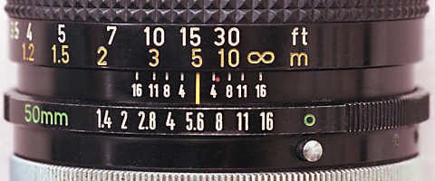
Most 35mm and medium format prime lenses and some zooms have depth of field (DOF) scales. Your camera's instruction manual states that if you stop down your lens, for example to f/8, everything at distances between the two f/8 DOF marks will appear to be "in focus." Of course, not exactly in focus. You may therefore ask the question, "How sharp is the image (what is its MTF?) at the DOF limit?" To answer these questions we begin with the diagram below, representing a lens with aperture a imaging an object at s on the film plane at d. .
An object at a distance s in front of the lens is focused at a distance d behind it, according to the lens equation: 1/d = 1/f - 1/s, where f is the focal length of the lens. If the lens were perfect (no aberrations; no diffraction) a point at s would focus to an infinitesimally tiny point at d. An object at sf , in front of s, focuses at df , behind d. At the film plane d, the object would be out of focus; it would be imaged as a circle whose diameter Cf is called its circle of confusion. Likewise, an object at sr, behind s, focuses at dr, in front of d. Its circle of confusion at d has diameter Cr.
The depth of field (DOF) is the range of distances between sf and sr, (Dr + Df ), where the circles of confusion, Cf and Cr, are small enough so the image appears to be "in focus." The standard criterion for choosing C (the largest allowable value of Cf and Cr) is that on an 8x10 inch print viewed at a distance of 10 inches, the smallest distinguishable feature is (allegedly) 0.01 inch. That was the assumption in the 1930's when film was much softer than it is today. At 8x magnification this corresponds to 0.00125 inches = 0.032 mm on 35mm film, close to the standard 0.03 mm used by 35mm lens manufacturers to calculate their DOF scales. If you've ever had a close look at a fine contact print from 4x5 or 8x10 film, you'll doubt that 0.01 inch feature size is a good criterion. Studies on human visual acuity indicate that the smallest feature an eye with 20:20 vision can distinguish is about one minute of an arc: 0.003 inches at a distance of 10 inches. But inertial prevails: 0.01 inch is universally used to specify DOF.
| Basic Lens and Depth of Field equations. | ||||||||||||||||
|
f50 = 0.72/C ; f20 = 1/C ; f10 = 1.11/Cf50 is familiar from film, lenses and scanners. f20 is interesting because it is the inverse of C. For C = 0.03mm, f50 = 24 lp/mm. An excellent lens for the 35mm format has f50 ~= 60 lp/mm.
The sharpness at the DOF limit for C = 0.03mm (typical for the 35mm format) is 24 lp/mm, about 40% of an excellent lens in focus (60 lp/mm). Not great!
You can determine the precise circle of confusion C for the depth of field scale on your lens with a simple procedure, using an equation derived from the box above.
|
For my old (medium format) chrome-barrel Hasselblad (Zeiss) lenses, C = 0.055 mm, corresponding to the same 0.01 inches on an 8x10 print, enlarged 5x for this format (nominally 6x6 cm, but actually 5.6x5.6 cm).
Zeiss has a good deal to say about DOF in Camera Lens News No. 1. Inadequate depth of field turns out to be their number one customer complaint. They state, "All the camera lens manufacturers in the world including Carl Zeiss have to adhere to the same principle and the international standard that is based upon it (0.03mm for the 35mm format), when producing their depth of field scales and tables." They summarize,
If the part of the scene at infinity is at all important in the image-- it's often visually dominant-- you'll be disappointed with the sharpness, which is only 40% that of a high quality lens in focus; about one third what the eye can distinguish. Merklinger recommends focusing at infinity-- you lose very little forward depth of field. I feel safe setting infinity focus opposite the far DOF mark corresponding to 2 stops larger than the actual f-stop setting (half the number). For example, if you are using f/8, it's safe to put the far f/4 DOF mark opposite infinity. It's a judgment call. When you make it, think about what parts of the image will be dominant. There is no rule to blindly follow.
Cbulge = bulge/f-stopFor a 0.08 mm bulge at f/5.6, Cbulge = 0.014mm. For a 0.2mm bulge at f/5.6, Cbulge = 0.036mm-- worse that the circle of confusion at the DOF limit. Pretty bad. That's why we sometimes need to stop down a little more than optimum.
To further confound you, film flatness is a function of time after winding the film. And it's different for 35mm and medium format. According to Robert Monaghan, film gets flatter if you wait up to 30 minutes after winding 35mm film, but according to both Mohaghan and Zeiss (in Camera Lens News No. 10) the bulge increases with time after winding medium format film: it's small at 5 minutes, significant at 15 minutes and maximum after 2 hours. One solid piece of useful information from Zeiss: the bulge is only half as much for 220 film as it is for 120. (That means I have to buy a new back if I go back to using my old Hasselblad; a great temptation.) The Zeiss rule of thumb is, " For best sharpness in medium format, prefer 220 type roll film and run it through the camera rather quickly." Temperature and humidity probably also affect flatness.
Oh yes, digital cameras don't suffer from film flatness problems. That's one reason why their performance is expected to exceed 35mm with only 6 to 10 megapixel sensors (multiplied by 3 when converted to RGB file formats). For much more detail on film flatness, I recommend Robert Monaghan's exhaustive discussion (with reader comments).
The smaller the aperture-- the larger the f-stop ( N )-- the more the image is degraded by diffraction. The equation for the Rayleigh diffraction limit, adapted from R. N. Clark's scanner detail page, is,
Rayleigh limit (line pairs per mm) = 1/(1.22*N *W )The MTF at the Rayleigh limit is about 9%. Most lenses for 35mm and larger cameras are aberration-limited-- relatively unaffected by diffraction-- at N = f/8 and below. The spatial frequencies for 10% and 50% MTF for diffraction-limited lenses are,
f10 = 0.77/( N *W ) ; f50 = 0.38/( N *W )The diameter of the corresponding circle, known as the Airy disk, is,
CAiry = 2.44*N *W (The 1.22 term in the Rayleigh limit comes from the radius.)Now here's the rub. If it weren't for diffraction, you could stop down a lens as much as you needed to get the depth of field you desired. But in the real world you reach a point where diffraction starts degrading the image more than misfocus. There is an optimum aperture that results in the best sharpness over a range of distances. But how to find that optimum isn't exactly common knowledge.
|
|
|
|
| f/4-f/8 | 2 f-stops | For example, if marks indicate f/4, close down to f/8. |
| f/11-f/16 | 1 f-stop | |
| f/22-f/32 | No change | |
| f/45 and above | Increase by 1 f-stop (!) | View camera territory, where diffraction takes a big bite out of sharpness. |
| Derivation of aperture for optimum sharpness over a range of distances | |||||||||||||||||||||||||||||||||||||||||||||||||||||||||||||||||||||||||||||||||||||||||||||||||||||||||||||||||||||||||||||||||||||||||||||||||||||||||||||||||||||||||||||||||||||||||||||||||||||||||||||||||||||||||||||||
|
| Equations for Total Depth of Field | |
|
Now let's look at Depth of Field for M ~= 1/20 at f/8 for several focal lengths, using Jonathan Sachs' Depth of Field Calculator set for 30 lp/mm resolution (the default).
|
|
|
|
|
|
|
| 20 mm | 400 | 319 | 536 | 217 | 54.2 |
| 50 mm | 1000 | 908 | 1113 | 205 | 20.5 |
| 100 mm | 2000 | 1904 | 2107 | 203 | 10.1 |
| 200 mm | 4000 | 3901 | 4104 | 203 | 5.1 |
| 1000 mm | 20000 | 19899 | 20102 | 203 | 1.0 |
For a specific format, depth of field, expressed as distance, is independent of focal length. But depth of field, expressed as a percentage of the distance to the subject (Total DOF/s %), is inversely proportional to focal length. It can be very small for long telephoto lenses.Using a long telephoto lens is an effective way of isolating a subject from busy, uncontrolled backgrounds without sacrificing actual depth of field.
| ||||||||||||||||||||||||||||||||
Since f/C is a constant, independent of format, depth of field is constant for constant aperture opening a. And since f-stop N = f /a,
Depth of field is constant when the f-stop is proportional to the format size, i.e., DOF is the same for a 35mm image taken at f/11, a 6x7 image at f/22, a 4x5 image at f/45 or an 8x10 image at f/90.This has important consequences when the lens sharpness becomes diffraction limited-- beyond around f/11 for 35mm; slightly larger for large formats. (High quality lenses become diffraction-limited at larger apertures. The f-stop at which diffraction becomes dominant increases rather slowly with format size.) A lens is likely to be diffraction-limited when a large depth of field is required; the larger the format, the more it must be stopped down; hence the more likely it is to be diffraction-limited. Once a lens is diffraction-limited its resolution is inversely proportional to its f-stop. This leads to a rather surprising observation.
When a lens is stopped down so to achieve a large depth of field, and is diffraction-limited, increasing the format size does not increase image sharpness, i.e., total resolution. For example, an 8x10 image taken at f/64 will be no sharper than a 4x5 image taken at f/32.This statement applies primarily to large formats (4x5 and above). For small formats, particularly 35mm, image sharpness is limited by film resolution. Fuji Provia 100F, one of the finest grained slide films, has resolution roughly equivalent to diffraction at f/16 ( f50 = 40 lp/mm; f20 = 70 lp/mm), but since the total system MTF is the product of the MTF of the individual components, you can see some improvement in overall sharpness for lens apertures as wide as f/8. You must choose film with care for optimum sharpness in the 35mm format. Film resolution also limits the sharpness of medium format images, but this is only noticeable on images larger than 13x19 inches-- the maximum for inexpensive consumer printers.
When large depth of field is needed, lenses usually have to be stopped down beyond their optimum aperture, especially for large formats, where very small apertures are required. Diffraction in digital cameras is discussed here.
If large DOF was required, it was obtained by using the camera's movements, particularly the tilt, which allows the plane of focus to be altered (via the Scheimpflug effect). Virtually all large format cameras have these movements; they are a major advantage. (Another, lesser, advantage is that sheet film tends have better flatness than roll films.) Few medium format cameras have these movements. (The Rollei SL66 was a rare and wonderful exception.) A few 35mm camera systems (most notably Canon) offer specialized lenses with movements. I love my old Canon FD 35mm f/2.8 TS lens, despite its manual aperture.
There is a sweet spot between large apertures, where lenses are aberration-limited, and small apertures, where they are diffraction-limited. Let's take a closer (but rough, qualitative) look. Good 35mm lenses tend to be sharpest around f/8, aberration-limited starting around f/5.6, and diffraction-limited starting around f/11. The total detail a lens can resolve at large apertures, where performance is aberration-limited, is relatively independent of format. It is a function of lens quality and design. A good lens can resolve about the same detail at f/5.6 for 35mm as for 4x5, where the image is much larger, but 4x5 images will have more detail because 35mm images are limited by film resolution.
The total detail a lens can resolve at small apertures, where performance is diffraction-limited, is proportional to to the format size and inversely proportional to the f-stop. A 35mm lens at f/11 resolves about the same total detail as a medium format (6x7) lens at f/22, a 4x5 lens at f/45, or an 8x10 lens at f/90. Resolutions at these apertures are roughly comparable to resolution of a high quality lens at f/5.6. (Disclaimer: this estimate is very rough! Variations between lenses make a huge difference.)
The sweet spot-- the range of apertures with excellent sharpness, tends to be between f/5.6 and the aperture corresponding f/11 for the 35mm format (f/22 for medium format, f/45 for 4x5, and f/90 for 8x10). It comprises about 3 f-stops for 35mm, 5 f-stops for medium format, 7 f-stops for 4x5, and 9 f-stops for 8x10.
The larger the format, the larger the sweet spot.Lenses have their optimum aperture-- their highest total resolution-- near the center of the sweet spot, typically around f/8 for 35mm, f/11 for medium format, f/16 for 4x5, and f/22 for 8x10. In practice, f/16 may be more practical for 4x5 and f/32 is more practical for 8x10 because depth of field is severely limited for large formats. Testing and experience will teach you which apertures are sharpest for your individual lens, but these numbers are good estimates. Optimum aperture is not sharply defined: for example, a good 4x5 lens with an optimum aperture around f/16 should produce excellent image quality between f/11 and f/32. Since large format lenses tend to be diffraction-limited at optimum aperture,
Total resolution at optimum aperture scales roughly with the square root of the format size for large formats.This rough but useful approximation applies to lenses only. When film losses dominate image quality, as it does for 35mm and medium format (recall, Fuji Provia 100F has MTF comparable to diffraction at f/16), total resolution scales linearly with format size. There is a greater advantage to larger formats.
I need to stress that the advantage of large formats is greatest when lenses are not stopped down to achieve extreme depth of field.
For very small formats-- for compact digital cameras with 11mm diagonal or smaller sensors (1/4 the size of 35mm), the sweet spot is extremely small. Lenses are aberration and diffraction-limited at the same aperture, around f/4 to f/5.6. They are severely diffraction-limited at f/8, where DOF is equivalent to f/32 or more in 35mm. (They rarely go beyond f/8.) But even though lens resolution is less than for 35mm film cameras, tiny digital cameras still produce very sharp images at f/4 and f/5.6 because their tiny pixels-- 4 micron spacing or less with no anti-aliasing filters-- have far better lp/mm resolution than 35mm film. Image resolution is almost entirely dominated by the lens.
Detail can be quite stunning in well-made large format images, particularly in very large prints-- beyond the 13x19 inch maximum size of most consumer digital printers. Large formats have little advantage for 8½x11 inch prints, although traditional 8x10 contact prints have a unique tonal beauty, particularly when made on special contact papers such as Azo. I've recently seen some incredibly sharp huge prints (over 40x50 inches) made from 8x10-- sharper than you could achieve with 4x5. But 4x5 is the largest practical format for carrying on hikes, and it has its own "sweet spot" for inexpensive flatbed film scanners such as the Epson 2450 and 3200. Even though these scanners have somewhat poorer resolution than dedicated film scanners, their resolution is sufficient to make sharp 32x40 inch prints from 4x5 film (the same magnification as 8x10 prints from 35mm). Of course I'd need a wide body printer, like the 24 inch wide Epson 7600, which could make extremely sharp 24x30 inch prints from 2450/3200 scans. Tempting!
| MTF equations for circle of confusion and diffraction. | |
|
好啊
| 欢迎光临 光电工程师社区 (http://bbs.oecr.com/) | Powered by Discuz! X3.2 |
 Set the lens's focus so the infinity mark is opposite the far DOF mark for the largest f-stop, Nmax , typically between f/16 and f/32. This is equivalent to setting sr to infinity.

 Because of phase effects implicit in OTF, the combined diffraction and focus error is not the product of the OTF's for diffraction and misfocus. (You can multiply MTF's for separate components, e.g., lens and flim, because phase is lost when you go from one to another.) The combined equation is relatively easy to solve numerically. It appears to work well in the limits of a c (diffraction dominant) and a c (misfocus dominant). Here is a plot of the individual and combined terms for N = f-stop = 22, C = 0.03mm and lambda (wavelength of light) = 0.000555mm (the same data as